Introduction
Everyone seems to have a slightly different take on the differences between Artificial Intelligence, Machine Learning, and Data Science. The following four articles cover some of the most common definitions.
As you read them, think about the differences and similarities of the definitions. Given the backgrounds of the various authors, whose opinions might you give more weight to?
- Michael Copeland writing for NVidia
- Bernard Marr writing for Forbes
- Vincent Granville writing for Data Science Central
- Simply Statistics Blog - The key word in “Data Science” is not Data, it is Science
Of particular note is this quote from the Granville article:
Earlier in my career (circa 1990) I worked on image remote sensing technology, among other things to identify patterns (or shapes or features, for instance lakes) in satellite images and to perform image segmentation: at that time my research was labeled as computational statistics, but the people doing the exact same thing in the computer science department next door in my home university, called their research artificial intelligence. Today, it would be called data science or artificial intelligence, the sub-domains being signal processing, computer vision or IoT.
As with most things in the realm of science, there tends to be a wide gap between how the media, government, and business sectors view a particular technology compared to how it’s viewed by the engineers and scientists using that technology.
For our purposes in this course, we’ll define these terms as follows:
Artificial Intelligence: The study of man-made “agents” that perceive their environment and take actions that maximize their chances of success at some goal.1
Machine Learning: A subfield within Artificial Intelligence that gives “computers the ability to learn without being explicitly programmed."2
Data Science: The study and use of the techniques, statistics, algorithms, and tools needed to extract knowledge and insights from data.3
MORAVEC’S PARADOX
In the 1980’s, Hans Moravec made the following observation, which came to be known as Moravec’s Paradox:
…as the number of demonstrations has mounted, it has become clear that it is comparatively easy to make computers exhibit adult-level performance in solving problems on intelligence tests or playing checkers, and difficult or impossible to give them the skills of a one-year-old when it comes to perception and mobility.4
So, while AI and machine learning algorithms can accomplish many tasks much better than humans can, any toddler can outperform even the most state-of-the-art neural network in picking out photos of their parents or pet cat.

Even though Moravec wrote about this over thirty years ago, the same sentiment persists in AI research today. In a 2016 interview, Dr. Sean Holden an AI researcher at Cambridge University, discussed the differences between human intelligence and artificial intelligence:
“Most AI researchers don’t try to solve the whole problem because it’s too hard. They take some specific problem and do it better. That’s not to say that the way humans think isn’t useful to AI, but working out how brains do things is hard. And there’s a difference in scale. Brains are doing things that are in some senses quite different from what AI researchers are currently attacking – I’d be ecstatic, for example, if I could build a robot that could put on a duvet cover.”6
Dr. Fumiya Iida, from the Machine Intelligence Lab at Cambridge, adds:
“We have hundreds of thousands of muscles in our body, so how can the brain control this? A computer can’t. Every fraction of a second you have to co-ordinate hundreds of muscles just to grab a cup, for example.”6
PREDICTION VS. INFERENCE
In machine learning, we are typically interested in doing one of two things: making inferences, or making predictions.
Inference: Given a set of data you want to infer how the output is generated as a function of the data.
Prediction: Given a new measurement, you want to use an existing data set to build a model that reliably chooses the correct identifier from a set of outcomes.7
This example explains the differences between those two goals:
Inference: You want to find out what the effect of Age, Passenger Class and, Gender has on surviving the Titanic Disaster. You can put up a logistic regression and infer the effect each passenger characteristic has on survival rates.
Prediction: Given some information on a Titanic passenger, you want to choose from the set {lives,dies} and be correct as often as possible.7
Classification Algorithms
Imagine that you’re a big fan of comic books. Over the years, you’ve read enough Marvel and DC comics that if I asked you to “classify” which universe Superman belonged to, you’d be able to confidently say, “The DC Universe”.
Or, let’s say you’ve eaten a lot of chocolate in your life. If I were to have you close your eyes and take a bite of chocolate, you might be able to accurately tell me if it was white chocolate, milk chocolate, semi-sweet, or dark.
These are both classification problems. Based on your prior knowledge or training regarding different groups, you can take an item and sort it into the correct group.
In machine learning, classification algorithms, (or classifiers), need to be trained before they can classify things on their own. We can train an algorithm by providing it with lots of examples from each group and telling it which attributes of those samples are important. The more examples we use to train our algorithm, the more accurate the classification of new items will be.
In the example below, we’re telling the algorithm “this is what a blue circle looks like”, or “this is what a green circle looks like”, etc…
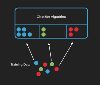
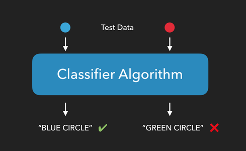
Once an algorithm has been trained, we can see how well it performs by providing it with test data consisting of new items it hasn’t seen yet, and checking to see if it can correctly predict which group the new items belong to.
The Iris Dataset
ABOUT THE DATA
For this example, we will use Fisher’s Iris Data.
The Iris dataset contains the length and width of the sepals and petals from 150 iris flowers across three different species of iris: Iris setosa, Iris versicolor, and Iris virginica.
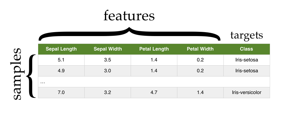
Each row in the Iris dataset represents the measurements of a single flower. We refer to each of these as a sample, observation, or instance.
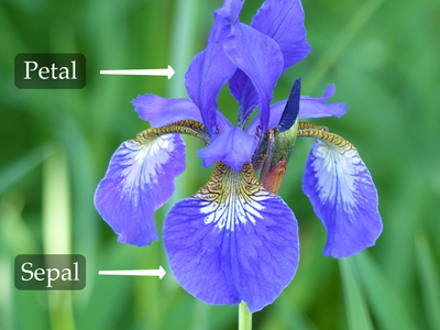
Each column in the Iris dataset represents a particular thing being measured about each flower. From left to right we have (in centimeters) the sepal length, the sepal width, the petal length, and the petal width. Each of these is referred to as a feature, attribute, measurement, or dimension.
The final column in the dataset is the species of the flower. This final column is often referred to as the target or class of the sample.
Classifiers
Classifier algorithms generally follow the same set of steps. Our goal is to create a classifier that can be provided with the measurements of petals and sepals, and then use that information to predict the species of iris flower we’re measuring.
Load data
The first thing we need to do is load our data. In most cases, there is some pre-processing that has to be done on the data in order to get it to the point where we can start working with it. Often you will need to normalize and encode variables.
In this case however, the data is provided to you in the exact format you need:
     sepal_length  sepal_width  petal_length  petal_width         species
0             5.1          3.5           1.4          0.2     Iris-setosa
1             4.9          3.0           1.4          0.2     Iris-setosa
2             4.7          3.2           1.3          0.2     Iris-setosa
3             4.6          3.1           1.5          0.2     Iris-setosa
4             5.0          3.6           1.4          0.2     Iris-setosa
..            ...          ...           ...          ...             ...
145           6.7          3.0           5.2          2.3  Iris-virginica
146           6.3          2.5           5.0          1.9  Iris-virginica
147           6.5          3.0           5.2          2.0  Iris-virginica
148           6.2          3.4           5.4          2.3  Iris-virginica
149           5.9          3.0           5.1          1.8  Iris-virginica
The csv file for the iris data can be found here. There are many ways to load data from a csv file, but one handy way is to use the read_csv function from the Pandas library:
import pandas as pd
url = "https://byuistats.github.io/CSE250-Course/skill_builders/ml_sklearn/machine_learning.csv"
data = pd.read_csv(url)
Split data
Next, we’ll randomly divide all of the samples into two groups. The first group will consist of our training data, or the samples we’ll use to train our classifier. The second group will consist of our test data, the data we’ll use to test our classifier.
There are many ways to do this, but if have our features (sepal and petal measurements) and targets (species names) in separate arrays, we can use the train_test_split function of the sklearn library to do this for us:
Note, that if you use pandas to load the csv file, you’ll have the data in a single pandas Data Frame. At some point you’ll need to split that data frame into two numpy arrays, one containing the features, and the other containing the targets.
Take a look at the Indexing and Selecting Data page in the Pandas user guide for more details and splitting the data, and the to_numpy function for converting to a numpy array.
Notice the transformation can be completed before the data is divided into test and training sets. Two numpy arrays can be passed to the train_test_split function to get two sets of arrays back. Alternatively, the data frame can be passed to the test_train_split, and then the test and training data is split into their feature and target components.
The following examples assume you’ve split the data into features and targets before passing it to test_train_split.
from sklearn.model_selection import train_test_split

# features = ... select the feature columns from the data frame
# targets = ... select the target column from the data frame

# Randomize and split the samples into two groups.
# 30% of the samples will be used for testing.
# The other 70% will be used for training.

train_data, test_data, train_targets, test_targets = train_test_split(features, targets, test_size=.3)
You could also use python’s built in libraries to randomly shuffle the data, and then use array slicing to split the data into test and training subsets. However if you do, make sure you do it in such a way that you still know which species goes with each set of measurements.
Train classifier
By providing the algorithm with training data, we allow it to create relationships between the features of a sample and its class. In the case of the Iris data set, we’re training our algorithm on how a given set of sepal and petal measurements correlate to the flower’s species.
sklearn has a classifier called GaussianNB which we can use to demonstrate this. GaussianNB is a “Naïve Bayes” classifier that assumes two things about our data:
- That the underlying features follow a continuous, normal distribution. (The Gaussian part)
- That each feature is statistically independent of every other feature. (The Naïve part)
Do you think both of these assumptions are true for the Iris data?
To train our classifier, first we create an instance of it, then we use the fit method to teach it about our data:
from sklearn.naive_bayes import GaussianNB
classifier = GaussianNB()
classifier.fit(train_data, train_targets)
Test classifier
Now that our classifier has been trained on how to classify iris flowers, it’s time to test it to see if it can correctly predict the species of flower from a set of measurements.
Note that it’s very important when testing our algorithm that we only test it on data that was not used to train it. Otherwise, we’re only testing it’s ability to remember training data. This is why we split the data into two groups.
To test our classifier, we’ll use the predict method and provide it with our test data. This method will return a list of predicted targets, one for each sample in the test data.
In our case, we’ll give it a list of petal and sepal measurements it has never seen before, and it will return a list of species predictions, on prediction for each sample in our test data:
targets_predicted = classifier.predict(test_data)
Assess classifier performance
Since we already know which type of iris each sample in the test data corresponds to, we can compare the predictions made by the classifier to the sample’s actual species and calculate how well our algorithm performs.
If m is the number of correct predictions made, and n is the total number of samples in our test data, then accuracy can be calculated as:
accuracy = m/n
So if our test data has 20 samples and the classifier predicts the correct flower species for 15 of them, then we would say our algorithm has an accuracy of 75%.
(Note that accuracy isn’t the best metric to use for evaluating classification algorithms. We’ll be looking at a few alternatives in the future.)
Summary
To summarize: we take our dataset and divide it in two parts: training data and test data. We use the training data to train the classifier to make classifications, then we use the test data to test how well our classifier performs.
If we have a classifier that performs well, we can use it with new data, samples whose groups we don’t know ahead of time, and the accuracy metric will give us some idea of how reliable those predictions are.
If our classifier performs poorly, we either need to provide it with more training data, modify or replace it, or select a different set of attributes to use as features.
CSE 450: Machine Learning & Data Mining is the class were you can build depth in Machine Learning and it’s applications.